

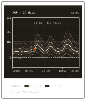
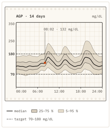
A continuous glucose monitor (CGM) that reads every 5 minutes collects 288 values a day, or 4,032 over the 14 days the international consensus recommends for a report. Every metric in this guide is computed from that list. The glucose bands are counts, glycemic variability is a mean and a spread, and the ambulatory glucose profile (AGP) is a set of percentiles. The calculations are short, and their reliability depends on the input, so the guide covers the input first.
Checking the glucose series before computing metrics
Each reading needs four things before it can count: a value, a unit, a measurement time and a code that says what was measured. Kymolog™ files CGM values as Observations in FHIR R4, the current release of Fast Healthcare Interoperability Resources. Each one is coded LOINC 99504-3, glucose in interstitial fluid, with the unit mg/dL. It names its sensor by unique device identifier (UDI) as well.
Check two things before computing any metric. The first is coverage: the consensus asks for 14 days of data, with the sensor active at least 70 % of that time. That much data correlates strongly with three months of mean glucose and time in ranges. The second is gaps: a missing reading should stay missing rather than repeat the last value, because a gap counted as in range inflates every share in the next section.
Measurement times need the same care. Each value should carry the time the sensor measured it, not the time the record reached a server. A receiver that uploads an hour of backlog sends 12 readings at once, and Kymolog files each under its own measurement time, so the series keeps its true spacing.
Check the units as well. A series that mixes mg/dL and mmol/L gives a meaningless mean, and the UCUM code on each value lets a script catch that before it averages anything.
Glucose bands and their consensus targets
Calculating time in range
To compute time in range, count the readings from 70 to 180 mg/dL in the reporting period and divide by the total: 204 of 288 readings is 70.8 %. The same count over the other four bands gives time below range and time above range.
| Band | mg/dL | Target, type 1 and type 2 diabetes |
|---|---|---|
| Very high (level 2) | above 250 | under 5 % of readings |
| High (level 1) | 181–250 | with very high, under 25 % above 180 |
| In range | 70–180 | over 70 % |
| Low (level 1) | 54–69 | with very low, under 4 % below 70 |
| Very low (level 2) | below 54 | under 1 % |
The bands and targets come from the international consensus on time in range: Battelino and colleagues, Diabetes Care 2019. Two targets are cumulative. Below 70 mg/dL counts the low and very low bands together, and above 180 counts high and very high together. Set one band's own share against either target and a day looks closer to target than it is.
The consensus sets looser targets for older or high-risk adults: over 50 % in range, under 1 % below 70 and under 10 % above 250. Pregnancy uses a narrower range, 63–140 mg/dL. The panel also notes that each 5 % increase in time in range is associated with clinically significant benefits.
The consensus states each target twice, as a share of readings and as time per day: over 70 % in range is more than 16 hours and 48 minutes. The two match only when the sensor ran all day, so report the share of readings with the data coverage beside it.
Figure 2 as a table
| Band | mg/dL | Readings | Share | Target |
|---|---|---|---|---|
| Very high | >250 | 12 | 4.2 % | <5 % |
| High | 181–250 | 63 | 21.9 % | see above 180 |
| Above 180, all | >180 | 75 | 26.0 % | <25 % |
| In range | 70–180 | 204 | 70.8 % | >70 % |
| Below 70, all | <70 | 9 | 3.1 % | <4 % |
| Low | 54–69 | 7 | 2.4 % | see below 70 |
| Very low | <54 | 2 | 0.7 % | <1 % |
| All readings | 288 | 100 % |
Glycemic variability: SD and CV
Glycemic variability, also called glucose variability, is the spread of readings around their mean. It is usually reported as two numbers, the SD and the CV.
Standard deviation
The standard deviation (SD) is in mg/dL. Subtract the mean from each reading, square the differences, add them up, divide by the number of readings minus one, and take the square root. For the twelve readings in Fig. 3 the mean is 156.0 mg/dL and the SD is 48.7 mg/dL.
SD tends to rise with mean glucose. An SD of 48.7 mg/dL around a mean of 156 describes a steadier day than the same SD around a mean of 110, so SD alone cannot compare two people.
Coefficient of variation
The coefficient of variation (CV) divides SD by the mean and states it as a percentage: 48.7 ÷ 156.0 × 100 = 31.2 %. Because it is relative to the mean, CV compares variability between people whose average glucose differs.
The consensus target is a CV of 36 % or less. It adds that some studies suggest a lower target, under 33 %, gives extra protection against hypoglycemia for people on insulin or sulfonylureas.
When you compute CV and SD from a study dataset, use the same period as the band shares, and say whether SD divided by n or by n − 1. Over 4,032 readings the choice barely moves the result; over twelve it moves SD by about 4 %.
Other measures of glucose variability
MAGE, the mean amplitude of glycemic excursions, takes another route. It averages only the swings from peak to nadir that are larger than one SD (Service and colleagues, Diabetes, 1970). It needs the full series in time order, which timestamped readings provide.
Figure 3 as a table
| Step | Working | Result |
|---|---|---|
| Readings | 00:00 112, 02:00 96, 04:00 84, 06:00 131, 08:00 204, 10:00 178, 12:00 146, 14:00 192, 16:00 163, 18:00 121, 20:00 238, 22:00 207 | n = 12 |
| Mean | 1,872 / 12 | 156.0 mg/dL |
| Sum of squared deviations | sum of (reading - mean) squared | 26,128 |
| SD (sample, n - 1) | square root of 26,128 / 11 | 48.7 mg/dL |
| CV | 48.7 / 156.0 × 100 | 31.2 % |
| Consensus target | CV | 36 % or less |
Bring a few days of CGM readings, or just the sensor class. The demo codes them as Observations and shows the study rows every metric here starts from.
Request a demoReading an ambulatory glucose profile
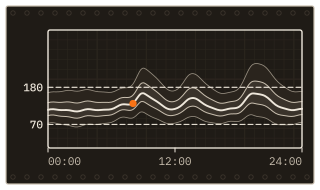
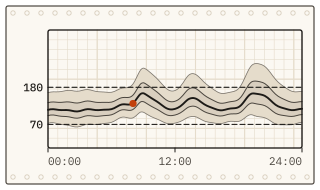
An ambulatory glucose profile folds 14 days of readings onto a single 24-hour day. At each time of day it plots the median of the readings taken then. Around the median sit two bands: the 25th to 75th percentile, and the wider 5th to 95th.
Building one from a coded series takes three steps. Group the readings by time of day across the 14 days, take the 5th, 25th, 50th, 75th and 95th percentiles of each slot, and draw the five curves.
The median shows the typical day, such as a rise after breakfast or a dip before dawn. The width of the bands shows variability at that hour: a wide band at 03:00 means glucose differs from night to night, even when each night's own trace looks stable.
The standardized AGP report puts this profile on one page with the core CGM metrics and their targets. These include the share of readings in each band, mean glucose, CV and the glucose management indicator (GMI), an estimate of A1C from mean glucose. The consensus recommends the AGP report as the template for CGM data.
Coding the results beside the readings
A computed metric is a result too, and LOINC has codes for the common ones. 97507-8 is average glucose in interstitial fluid over a reporting period, 97510-2 is the share of readings in range, and 97506-0 is GMI. The Kymolog CGM device type carries all three, so a summary can sit as an Observation next to the readings it came from.
Each summary and each reading names its sensor and its period, so a reviewer can recount any number in a report from the rows beneath it. The page on CGM data analysis shows how those readings are captured and filed in the EHR.
For the clinical side of a CGM study, such as A1C results drawn in the lab and insulin orders, Clinical Extract extracts the EHR's own records.
Before you report a CGM metric
- Count the days and the share of time the sensor was active: 14 days, at least 70 % active.
- Leave gaps empty, and report how many readings the period should have held against how many it did.
- Check that every value carries the same unit before averaging.
- Compute the band shares, SD and CV over the same period.
- State whether SD divided by n or n − 1, and which target set you compared against.